Machine Learning for Threat Classification

The Importance of Class Imbalance, Explainability and Ensemble Methods

Written by Yamineesh Kanaparthy.

Generated using Craiyon AI art generator

Introduction

Cybersecurity is a constantly evolving field, with new threats emerging all the time. To stay ahead of the curve, security teams need to be able to quickly and accurately identify and respond to threats. Machine learning can play a vital role in this, by providing a way to automate the detection of threats. This article focuses on the need and techniques for Class Imbalance, Explainability and best practices in the Modelling process. To demonstrate the detailed techniques using Python, Netflows captured in the UNSW-NB15 Dataset were used. Please refer to the source for feature description and data collection approach.

The Imbalance Problem

One of the challenges of using machine learning for cybersecurity is that the data is often imbalanced. This just means that there are many more examples of normal traffic than there are examples of malicious traffic. This is because,

1. The number of malicious attacks is relatively small compared to the number of normal connections. So, most connections are normal, and only a small percentage of connections are malicious.
2. Malicious attacks are often very short-lived. This means that there may not be enough data to train a machine learning model to identify malicious traffic.
3. Malicious actors are constantly changing their methods. This means that the data that is used to train a machine learning model may quickly become outdated. This can make it difficult for machine learning models to learn to identify malicious traffic.

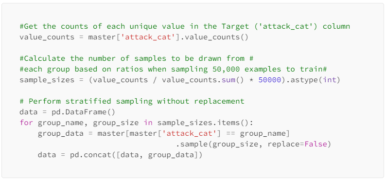
A Stratified approach to Sampling

Imagine you are trying to build a machine learning model to classify coins as heads or tails. If you only use heads to train the model, the model will only be able to learn to classify heads. Stratified sampling is a technique to ensure that the proportion of examples of each class (heads and tails) in the training data, is representative of the actual observations/ outcomes. Stratified sample is achieved by dividing the data into groups, based on the class label. Then, a random sample is taken proportionally from each group. Here is how this can be implemented.

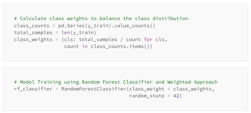
Class Balancing using Weighted Approach

Class imbalance is a common problem in machine learning, but it can be especially challenging in cybersecurity. Class balancing is a measure to ensure that the model is not biased towards one class or another. One way is to use a weighted approach. In this approach, you assign different weights to the classes during the training process. The weights are usually inversely proportional to the class frequencies. This means that the minority class gets a higher weight, making the model pay more attention to it during training.

For example, if there are 100 examples of normal traffic and 10 examples of malicious traffic, then each example of malicious traffic would be weighted 10 times more than each example of normal traffic. This would help to ensure that the machine learning model learns to identify malicious traffic even though there is less data for that class. Below is an example of how the class weights are calculated to balance the distribution and used in building the classifier.

SMOTE (Synthetic Minority Over-sampling Technique)

SMOTE is a data augmentation technique specifically designed to address class imbalance. It creates synthetic (not in the original data) examples for the minority class by generating new instances that are similar to the existing minority class samples. This is done by selecting a sample from the minority class, identifying its k nearest neighbors, and then creating new instances along the line segments connecting the chosen sample and its neighbors. Here is how it can be implemented in Python.

Explainability is Very Important

Generated using Craiyon AI art generator

Once a machine learning model has been trained, it is important to understand how the model is making its predictions. This can be done by looking at the feature impact of the model. The feature impact shows how much each feature contributes to the model’s prediction.

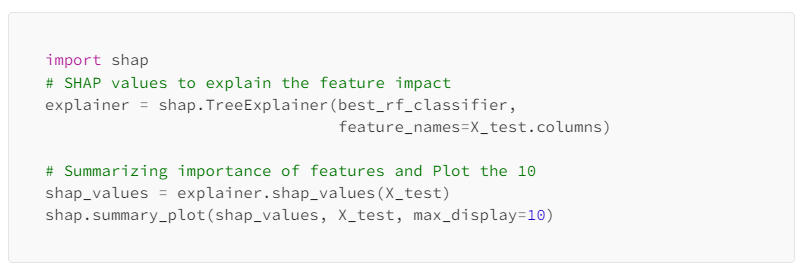
SHAP values are one way to explain the predictions of a machine learning model. They are calculated by measuring the impact of each feature on the model’s prediction, both individually and in combination with other features. One remarkable feature of SHAP values is that they don’t require the target values for generating explanations. SHAP values are based on cooperative game theory and provide a way to attribute the contribution of each feature to the difference between a model’s prediction and the average prediction across all possible feature combinations.

SHAP also offers specific tree explainer algorithms, such as the “TreeExplainer,” which breaks down the predictions of ensemble models into contributions from individual features. It is also important to understand that SHAP values only quantify feature contributions but do not provide a complete understanding of the model’s decision-making process, particularly in cases where interactions between features are crucial. Despite this, it is a useful tool for enhancing model interpretability and transparency.

For instance, the SHAP summary plot below reveals the significant influence of certain features on threat classification. Notably, ‘ct_srv_src’ (the count of connections sharing the same service and source address in every 100 connections), ‘sbytes’ (transaction bytes from source to destination), and ‘service_dns’ (when the service type is DNS) emerge as the top three contributors, wielding the most substantial impact on the threat classification outcome.

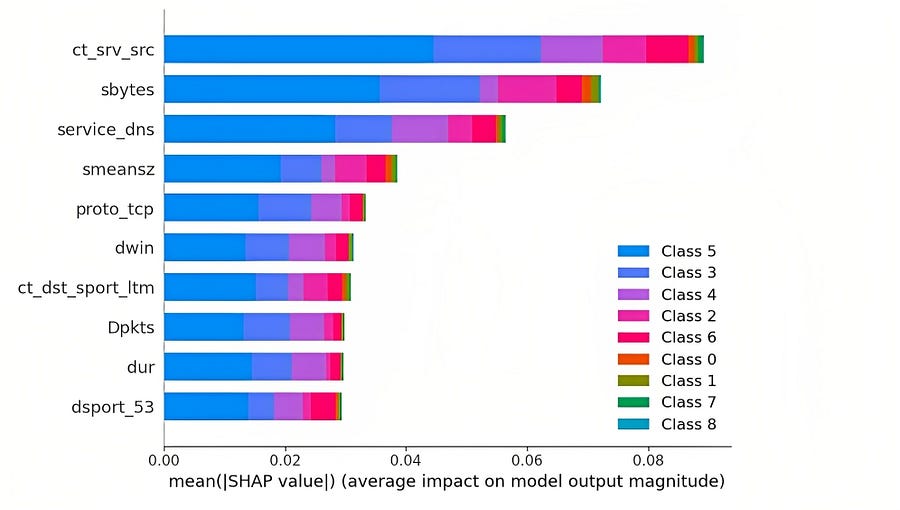
Top 10 Features and their impact on each class

The Feature impacts can also be examined for a specific class to understand the varying effects of features for classifying a threat differently. In the below example, in classifying Denial of Service attacks, sbytes, (source to destination transaction bytes), ct_srv_src (No. of connections that contain the same service and source address in 100 connections) and smeansz (Average packet size transmitted by the source) have had the highest impact.

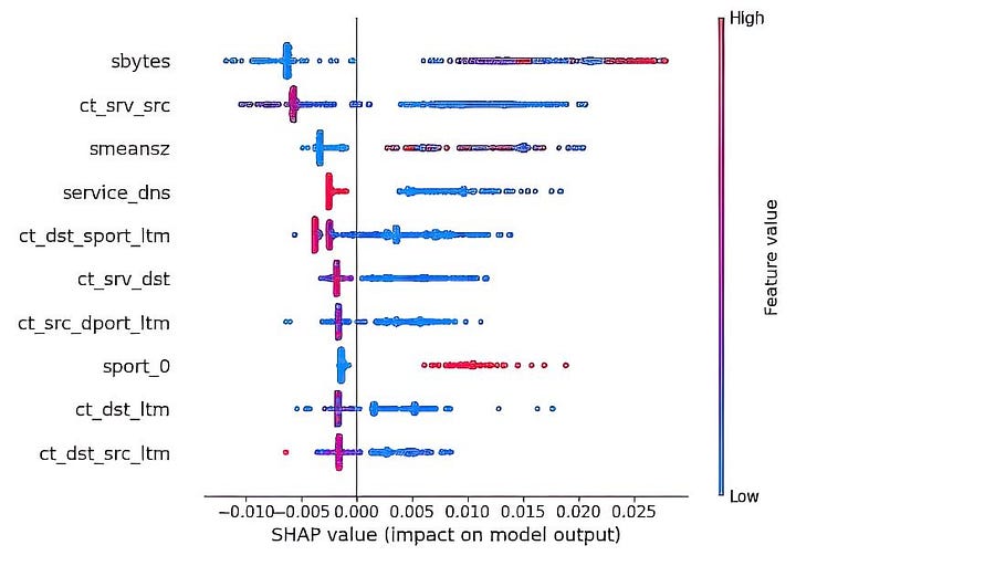
Top 10 Features in identifying a DoS attack

A SHAP force plot is also a useful tool for understanding how a model makes decisions. The plot visualizes the relative importance of each feature in a prediction and shows how each feature contributes to the prediction, both positively and negatively. They can be used to identify features that are most important to the model, to identify interactions between features, and to debug models that are making unexpected predictions. “Higher” (in red), indicates that the feature has a positive impact on the prediction and “Lower” (in blue), indicates a negative impact. f(x) represents the model’s prediction for a specific instance. It is the sum of the base value and the contributions of individual features (SHAP values) for that instance. Mathematically, it can be expressed as,

f(x) = Base Value + Σ(SHAP Value for each feature).

Here is an example of using a force plot. In this context, the model’s prediction of a relatively low threat likelihood (0.01) is influenced by the value of sbytes (534), which is significantly above the typical baseline value (0.008356). Baseline value refers to the expected or average prediction of the model when all features are set to their baseline values (often the mean values for continuous features or the mode values for categorical features). This suggests that the sbytes(Source-to-destination byte count) being transmitted in the range of 534 might be contributing to the model’s prediction that this specific instance is less likely to be a threat.

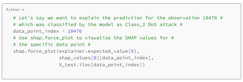
Force plot explaining the feature importance

Removing Highly Correlated Features requires Awareness

Free Stock photos by Vecteezy

As a data scientist, it is generally a good practice to remove highly correlated features from a machine learning model. However, this approach also needs caution, particularly when dealing with Netflow data. During the modeling process, we can observe that most features in Netflow data highly correlate. Some contributing reasons for this behavior are,

1. Traffic Patterns and Behaviors: Network traffic often follows specific patterns and behaviors. For example, communication between specific IP addresses and ports might be associated with certain types of services or applications. These patterns can result in high correlations among features related to the same services or applications.
2. Network Infrastructure: The network’s architecture and design can lead to correlations among features. Subnets, VLANs, and other network segmentation strategies can cause certain features to be highly correlated due to the structured nature of the network.
3. Protocols: Different network protocols have distinct behaviors and communication patterns. Features related to specific protocols can exhibit high correlations as a result.
4. Traffic Volume: Features such as packet counts, byte counts, and duration of communication can be correlated because they are often related to the same communication events. For example, a higher number of packets might correspond to a longer duration of communication.
5. Sampling and Aggregation: Netflow data might sometimes be collected in a sampled or aggregated manner, which can lead to correlations. Aggregating data over time intervals or grouping data by certain attributes can result in correlated features.

Removing some highly correlated features can make a model less accurate. This is because highly correlated features may still contain distinct information about the state of a network. When these features are removed, the model may lose some of the information that it needs to identify potential attacks and hence it is important to understand the correlations.

For example, let’s say we have a machine learning model that is trained to detect DDoS attacks. The model is trained on a dataset of features that describe the network traffic patterns leading up to a DDoS attack. Some of these features such as the ‘number of packets per second’ and the ‘size of the packets’ may be highly correlated. If we remove these highly correlated features from the model, the model may be less accurate because it will no longer have all of the information it needs to distinguish between normal network traffic and DDoS traffic.

Using dimensionality reduction techniques like Principal Component Analysis (PCA) can help in mitigating multicollinearity and improving model stability while retaining relevant information.

It is also in making these decisions where Domain knowledge plays a critical role.

Ensemble Methods are a good starting point

Free Stock photos by Vecteezy

Ensemble machine learning is a powerful tool that can perform well in classifying a threat in cybersecurity. This is because,

1. Cyber threats constantly evolve, leading to variations in attack patterns. Ensembles can handle this variability by capturing different aspects of attacks through their diverse base models. This helps in generalizing across various types of threats.
2. Ensembles employ multiple different base models, which could be based on different algorithms, hyperparameters, or subsets of data. This diversity reduces the risk of overfitting and increases the ensemble’s ability to capture a wide range of threat patterns.
3. Ensembles tend to be more robust to noisy or outlier data points since individual errors are balanced out by the combined decision of multiple models.

By using the techniques discussed in this article and combining them with standard modeling best practices, security teams can build accurate and reliable machine learning models that can help to protect their organizations from malicious attacks.

About the Author

Peer Reviewed By

References

1. Moustafa, Nour, and Jill Slay. “UNSW-NB15: a comprehensive data set for network intrusion detection systems (UNSW-NB15 network data set).” Military Communications and Information Systems Conference (MilCIS), 2015. IEEE, 2015.
2. Moustafa, Nour, and Jill Slay. “The evaluation of Network Anomaly Detection Systems: Statistical analysis of the UNSW-NB15 dataset and the comparison with the KDD99 dataset.” Information Security Journal: A Global Perspective (2016): 1–14.
3. Moustafa, Nour, et al. “Novel geometric area analysis technique for anomaly detection using trapezoidal area estimation on large-scale networks.” IEEE Transactions on Big Data (2017).
4. Moustafa, Nour, et al. “Big data analytics for intrusion detection system: statistical decision-making using finite dirichlet mixture models.” Data Analytics and Decision Support for Cybersecurity. Springer, Cham, 2017. 127–156.
5. Sarhan, Mohanad, Siamak Layeghy, Nour Moustafa, and Marius Portmann. NetFlow Datasets for Machine Learning-Based Network Intrusion Detection Systems. In Big Data Technologies and Applications: 10th EAI International Conference, BDTA 2020, and 13th EAI International Conference on Wireless Internet, WiCON 2020, Virtual Event, December 11, 2020, Proceedings (p. 117). Springer Nature.
6. Chawla, N. V., Bowyer, K. W., Hall, L. O., & Kegelmeyer, W. P. (2002). SMOTE: Synthetic Minority Over-sampling Technique. Journal of Artificial Intelligence Research, 16(16), 321–357. https://doi.org/10.1613/jair.953
7. Pinsky, Eugene. (2018). Mathematical Foundation for Ensemble Machine Learning and Ensemble Portfolio Analysis. SSRN Electronic Journal. https://doi.org/10.2139/ssrn.3243974
8. Shapley Values. (n.d.). C3 AI. https://c3.ai/glossary/data-science/shapley-values/#:~:text=However%2C%20its%20downside%20is%20complexity
9. Hofstede, R., Celeda, P., Trammell, B., Drago, I., Sadre, R., Sperotto, A., & Pras, A. (2014). Flow Monitoring Explained: From Packet Capture to Data Analysis With NetFlow and IPFIX. IEEE Communications Surveys & Tutorials, 16(4), 2037–2064. https://doi.org/10.1109/comst.2014.2321898